Our regime model flagged bear markets weeks early. Trading on it still lost money.
A hidden-Markov regime model turned "stressed" a median of 52 sessions before the Nasdaq-100 fell below its 200-day average. Cutting exposure on that signal still lost to buy-and-hold, because stress readings tend to arrive after the damage, when rebounds are more likely. And in summer 2026, two versions of the model disagreed completely.
Rayana AI Research · Nov 12, 2026
Regime models promise something every investor wants: a signal that the market has shifted from calm to dangerous, early enough to act on. We built one, tested it the strict way, and it passed the test most write-ups stop at: it turned early. It failed the test that matters, which is whether acting on it pays.
The model
A hidden Markov model (HMM) assumes the market moves between a few unobserved states, each with its own typical behavior, and estimates which state it's in from what it can observe. Ours watches four daily measures on point-in-time Nasdaq-100 members:
- Trend: QQQ's 5-day return.
- Volatility: QQQ's 21-day realized volatility.
- Dispersion: how far individual stocks' own moves spread apart, after removing the market's.
- Crowding: how much stocks are moving together.
It sorts days into three states. The stress state is the one with high volatility, high crowding and weak trend. The output is a daily probability that the market is in stress, from 0 to 1.
No look-ahead. This is where regime backtests most often cheat. The model's parameters are re-estimated every 21 sessions using only the data available at that point, and each day's reading uses only that day's and earlier observations. The sample runs from October 2011, with readings from October 2013 (after a two-year warm-up) to October 30, 2026.
The good news: it turns early
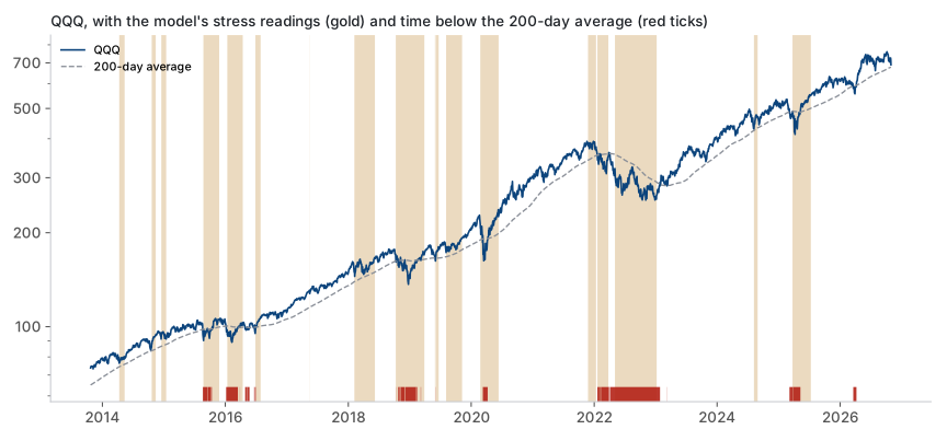
We measured lead time against a simple, widely used bear-market marker: QQQ closing below its 200-day moving average. There were 29 such crossings in the sample.
- The model's stress probability crossed 0.5 before 26 of the 29, a median of 52 sessions earlier.
- A two-state version of the model led all 29, a median of 59 sessions earlier.
That sounds like a strong early-warning system. Two caveats show it's less than it looks:
- The crossings cluster. The 29 come from about six selloffs (2015–16, late 2018 into 2019, early 2020, 2022–23, spring 2025 and March 2026), with the index whipsawing around its average several times in each. In 12 of the 26 "leads", the model had already been in stress for the whole 60-session window we checked.
- It's in stress often. The three-state model read stress on 28% of all days, and the two-state version on 50%. A signal that's on that often will precede most bad periods. Of the 19 separate times the three-state model entered stress, 7 were not followed by a 200-day break within the next 60 sessions.
The bad news: acting on it loses
The natural way to use a stress probability is to scale exposure by it: if the model says 70% stress, hold 30% of a normal position. We applied that to QQQ using each day's reading for the next day's position, with cash earning nothing:
| Strategy, Oct 2013 – Oct 2026 | Return per year | Worst drop | Sharpe | MAR | Avg exposure |
|---|---|---|---|---|---|
| Buy and hold QQQ | 18.8% | −35.1% | 0.92 | 0.54 | 100% |
| Scale by stress (3-state model) | 11.4% | −27.5% | 0.82 | 0.42 | 72% |
| Scale by stress (2-state model) | 7.2% | −17.4% | 0.74 | 0.41 | 50% |
| Scale by stress (trend and volatility only) | 10.4% | −19.7% | 0.84 | 0.53 | 69% |
MAR is annual return divided by the worst drop: return per unit of pain. All figures are before trading costs.
Every version cuts the worst drawdown, and every version gives up more return than the drawdown it saves. None beats buy-and-hold on Sharpe or MAR. A dollar held from October 2013 grew to $9.37; the three-state overlay turned it into $4.07.
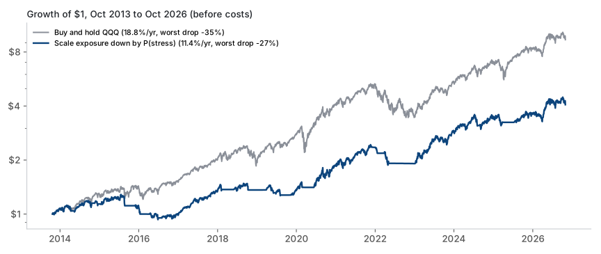
The flat stretches in that chart show why. The overlay did step aside for most of 2022's slide. But it also sat out the recoveries in 2016, 2019 and 2020, and those cost more than the protection was worth.
Why: stress readings arrive after the damage
The table that explains it compares what happened before and after stress days:
| Previous 21 sessions, QQQ | Next 21 sessions, QQQ | Next 21 sessions positive | |
|---|---|---|---|
| Days the model read stress | −0.2% | +2.3% | 69% |
| Days the model read calm | +2.3% | +1.4% | 67% |
The model reads stress after a rough patch: the month before a stress day was flat to down. And the month after was better than average. High volatility and crowding are what a selloff looks like once it has happened, and sharp selloffs are often followed by sharp rebounds. A model that measures turbulence is a good description of the present. As an exit signal, it tends to fire close to the bottom.
We found the same pattern with a very different tool. Our momentum-crash monitor showed that the stocks hit hardest on crash days went on to do better than usual over the following month.
Summer 2026: two versions, two answers
The out-of-sample test came in June and July 2026. In August, we ran the model trained on market history back to 2004. Its stress probability jumped from 0.17 on June 15 to 0.98 on June 17, and stayed above 0.5 for 23 sessions, until July 20. Throughout, QQQ traded within about 7% of its early-June high. Then, on July 29, QQQ hit its low for the move, down 11% from that high, and the model read 0.001: almost perfectly calm. QQQ never fell below its 200-day average. That's the timing problem above, playing out live.
For this note we re-ran the model on a shorter history starting in 2011, the same data behind every other number here. That version read calm the entire summer, never rising above 0.12. Changing the random starting points and the number of fitting attempts made no difference. The difference came from the training history alone.
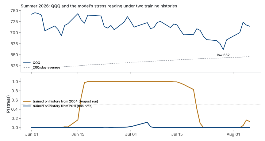
Neither version was "right" in a way you could have used. One raised a confident alarm at the wrong time; the other never raised one. A de-risking rule built on either would have depended on how far back someone chose to start the data, a choice that should not matter. Through October 30, QQQ still hadn't closed below its 200-day average, so this cycle has no new bear onset to grade the lead time against.
The extra inputs didn't help either
We built the model with dispersion and crowding because we expected them to sharpen it. They didn't. A version using only trend and volatility did as well on risk-adjusted terms (MAR 0.53 against 0.42), with a smaller worst drop. The added inputs made the model more complicated without making it more useful.
How we use it
The regime model is a diagnostic. It isn't wired to any portfolio weight, and on this evidence it shouldn't be. We keep it because it does what it actually measures, describing how turbulent the market is right now, and that context is useful when reading other signals.
Takeaways:
- Leading isn't the same as being useful. The model turned a median of 52 sessions before 200-day breaks, but it reads stress so often that leading most bad periods is easy.
- Stress readings mark turbulence that has already happened. On average, the next month was better after stress days than after calm ones.
- Scaling exposure by stress cut drawdowns, but cut returns by more. No version beat buy-and-hold on a risk-adjusted basis, before costs.
- The regime label depended on the training window. Two reasonable versions disagreed completely about summer 2026. That instability alone rules out trading on it.
Method notes: Gaussian hidden Markov model with three states (two-state results shown for comparison), fitted with multiple random restarts. Inputs computed daily from point-in-time Nasdaq-100 constituents and QQQ. Parameters re-estimated every 21 sessions on an expanding window, after a 504-session warm-up; daily readings use a forward filter only, with no smoothing or future data. Readings from October 23, 2013 to October 30, 2026. Lead time measured against QQQ closes below its 200-day simple moving average, looking back up to 60 sessions for the first stress reading above 0.5. The overlay holds QQQ at (1 − yesterday's stress probability), with cash at zero return and no trading costs. The summer-2026 comparison uses the model's August 7, 2026 run, trained on history from 2004. All results are historical and hypothetical.